Billions of real numbers, and nobody quite knows how they work. That’s the state of things. We can probe, decompose, and visualize what’s happening inside a transformer, but the gap between “these features fired” and “this is what the model is doing” remains wide open.
The previous post covered what happens when you hit enter. Tokens flow through layers, probabilities get shaped, text comes out. System prompts anchor the model in activation space. Temperature controls how tightly it follows that anchor.
This post goes one level deeper, into the model’s layers. What are those activations? What shape do they take?
For this experiment, I used a well-documented workflow built around Google’s Gemma 2 2B model and the Gemma Scope residual stream SAEs. These are Sparse Autoencoders trained by Google on Gemma’s residual stream activations. They act as auxiliary models that decompose dense internal states into sparse, more interpretable features. The tools are Gemma-specific but the concepts apply to any transformer model.
Vectors: The Model’s Internal Language
Think about the gas laws. Compress a gas, it gets hotter. The macroscopic behavior is simple. Underneath, there’s a seething mass of atoms bouncing around, and the real explanation lives in those microscopic dynamics.
Neural networks work the same way. The macroscopic behavior is “the model talks about France.” The microscopic dynamics are activation patterns flowing through 2304-dimensional space. We’re mapping the microscopic level. That’s what makes this worth doing.
A vector is a list of numbers. In Gemma 2 2B, the vector at each token position is a list of 2304 numbers. That’s the model’s d_model dimension, its internal working width.
No single number in that list is human-readable. But the pattern across all 2304 numbers encodes what the model “knows” at that point in the text.
When Gemma processes "The capital of France is", the vector at the last token position holds a pattern that implicitly represents “France,” “capital,” “geography,” “Paris is likely next.” All at once, smeared across 2304 dimensions.
It’s like coordinates in a 2304-dimensional space. We can’t visualize that. We can barely reason about it. But the model navigates this space constantly during generation, and every decision it makes is a movement through it.
How vectors flow through the model during this experiment:
- A prompt goes in. The model processes it token by token
- At layer 12, each token has a vector of shape
(2304,). That’s the residual stream
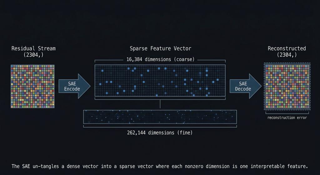
- The SAE takes that 2304-number vector and decomposes it into a sparse vector of 16,384 (coarse, fewer broader buckets) or 262,144 (fine, more narrower buckets) numbers, where most are zero and the nonzero ones correspond to interpretable features
- A steering vector is also
(2304,). Adding it to the residual stream shifts the pattern toward a concept
Steering is literally vector addition. Nudging coordinates in a space we can’t see.
The Residual Stream: The Highway Everything Rides On
The residual stream is the main data highway through the transformer. One vector, 2304 numbers, that persists across all 26 layers.
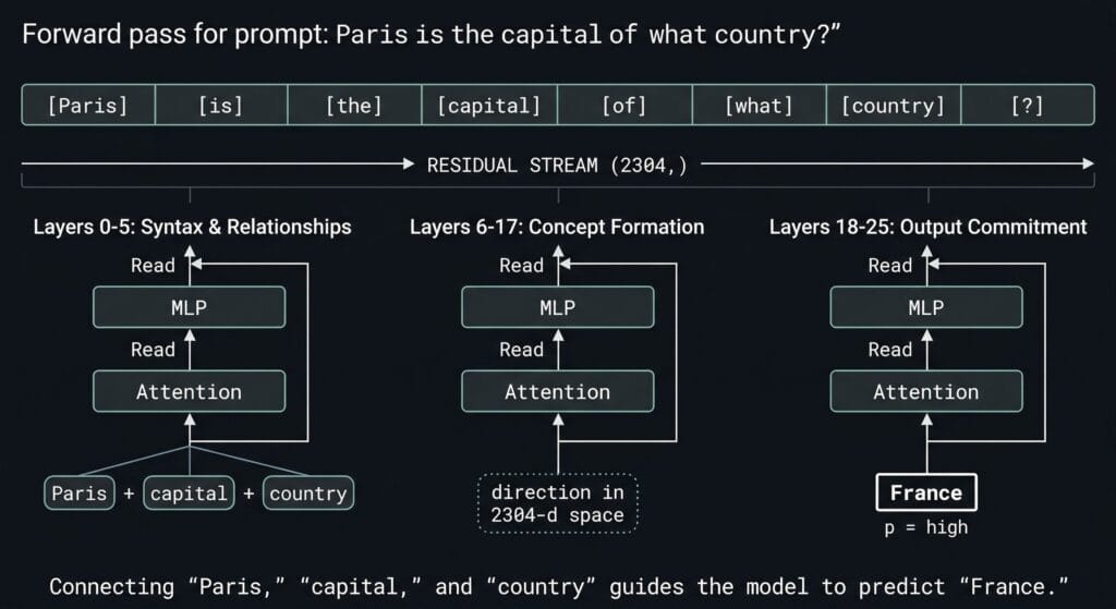
The key insight – each layer doesn’t replace the vector. It adds to it.
- Token embedding creates the initial vector
- Layer 0’s attention reads the vector, computes something, and adds its output back
- Layer 0’s MLP reads the updated vector, computes something, and adds its output back
- Layer 1 does the same
- All the way to layer 25
- The final vector gets mapped to token probabilities
It’s called “residual” because of this additive pattern. Each layer contributes a small change, a delta, and the stream accumulates all of them. Nothing gets thrown away. The vector at layer 25 contains every modification from every layer before it.
This additive pattern is also why the activation space anchoring from the previous post works, and why steering vectors work. More on steering in a future post once I finish that experiment.
Why Layer 12?
Gemma 2 2B has 26 transformer layers, numbered 0 through 25. I’m hooking into layer 12. Roughly the middle of the network.
The hook point is blocks.12.hook_resid_post, capturing the residual stream after layer 12 finishes processing.
Why mid-network?
This isn’t arbitrary. Google’s Gemma Scope team trained Sparse Autoencoders specifically on this layer’s residual stream. Both the 16K-width (coarse) and 262K-width (fine) SAEs in this experiment were trained to decompose layer 12 activations into interpretable features.
Middle layers carry more abstract semantic structure, and later layers get closer to output commitment. In practice, models distribute these functions across layers more unevenly than clean diagrams suggest, but the heuristic holds well enough that mid-network layers are the standard target for interpretability work. Layer 12 sits in the range where concepts like “France” are abstract enough to be meaningful, but still early enough to be malleable.
The SAE IDs make this explicit: layer_12/width_16k/average_l0_82 and layer_12/width_262k/average_l0_121. The average_l0 number is the average count of nonzero features per input. That’s the sparsity level. The 16K SAE activates roughly 82 features out of 16,384 on average. The 262K SAE activates about 121 out of 262,144. The vast majority of features are zero for any given input, and the nonzero ones are the signal. Everything in this experiment is anchored to layer 12.
What Does “Mapping Activations” Mean?
- Coarse (16K SAE): fewer features, each covering more conceptual ground.
- Fine (262K SAE): more features, each with higher resolution on specific facets.
An SAE decomposes a single 2304-number vector into thousands of sparse components called features.
Most of them have nothing to do with France. They encode punctuation patterns, sentence structure, token frequency artifacts, general semantic scaffolding. The task is figuring out which ones are France-specific.
Geoffrey Hinton uses a good analogy for this in a recent Star Talk interview.
Prompt “cat” and a bunch of micro-features activate: animate, furry, whiskers, pet, predator.
Prompt “dog” and a similar but different set fires: animate, furry, pet, predator, but not whiskers, and with different strengths.
The macro-concept lives in a distributed pattern of micro-features. That’s exactly what the SAE is decomposing, highlighting what’s already there, like an MRI with contrast dye injected. The structure was always in the tissue. The dye just makes it visible.
So back to the actual numbers. The 2304-number residual stream tangles all these micro-features together. The SAE takes that tightly packed, dense circuitry and expands it out into a much wider space so we can see which patterns actually fired.
How sparse is sparse?
The coarse SAE was trained so that a typical input activates only around 82 features out of 16,384, though the exact count varies by prompt. The important point is that the representation stays sparse: most features remain at or near zero, and only a small subset carries the useful signal. What goes in is tangled and unreadable. What comes out is mostly silence, with a few features we can actually interpret.
Here’s what that actually looks like. When I fed "The capital of France is" through Gemma and decomposed layer 12 through the coarse SAE, the top activating features were:
Feature #3999:   mean activation 3.67, selectivity 0.97  ← France (strongest signal)
Feature #11333:  mean activation 4.48, selectivity 0.89  ← France-related
Feature #9473:   mean activation 1.21, selectivity 0.88  ← France-related
Feature #14805:  mean activation 1.24, selectivity 0.86  ← France-related
Feature #6211:   mean activation 1.27, selectivity 0.86  ← France-related
...
Feature #6,004:  activation 0.00                         ← silent
Feature #6,005:  activation 0.00                         ← silent
[~11,000 more at zero]
The key column we should focus on is selectivity:
how exclusively does a feature fire on France prompts versus neutral ones?
Feature #3999 scores 0.97 – Meaning it almost only fires on France-related input. Notice #11333 actually fires harder (mean 4.48 vs 3.67) but has lower selectivity, it bleeds into some neutral prompts too. A feature that fires on everything isn’t telling you anything useful, no matter how loud it is.
I chose France as a sanity-check target because the interpretability method was already grounded in prior work, and Gemma Scope gave me a validated SAE setup to test whether my own pipeline recovered coherent structure.
The experiment follows standard A/B logic. Run ~400 prompts through Gemma,
half France-themed prompts , half neutral filler prompts 200 Each
Capture layer 12 activations for both sets. Decompose both through the same SAEs.
Then compare features that fire consistently on the France set but stay quiet on the neutral sets
now we have the candidates for “France features.” Features that fire on everything else can be safely considered noise.
I ran this experiment through both the coarse (16K) and fine (262K) SAEs because the zoom/resolution level matters.
The 16K SAE might compress everything France-related into a single feature, one bucket for the whole concept. The 262K SAE has 16x more features, so it can split that same signal into finer slices: one feature fires on cuisine prompts, another on geography, another on history. Same concept, different zoom levels.
Two Resolutions, One Concept
The 16K SAE (coarse) might give you one feature — call it #3999 — that broadly responds to “France.” One fat bucket for the whole concept.
The 262K SAE (fine) might split that same concept into multiple features. #86473 fires on a subset of France prompts. #249284 fires on a different subset. #243533 on another. Each one potentially encoding a different facet (cuisine, geography, landmarks, language) though we don’t know which facets they are yet. More on that problem in a minute.
This is hierarchical feature decomposition.
Same logic as hand-designing a vision network:
- Edges combine into shapes
- Shapes combine into objects
- Objects together in a scene change the meaning again (meaning as in what regions get excited to infer what it is)
Each layer builds on the last. Nobody hand-wires a transformer, but the same hierarchy emerges from training.
The coarse SAE finds the whole object. The fine SAE finds the parts or the edges. Nobody designed these decompositions. They emerged from training.
The cross-resolution mapping step figures out which fine features correspond to which coarse features. It measures two things:
- Activation correlation: do they fire on the same prompts? (behavioral evidence)
- Decoder cosine similarity: do their decoder vectors point in the same direction in the 2304-dimensional residual stream? (geometric evidence)
s fire together but point in different directions. They might encode co-occurring concepts rather than the same concept at different zoom levels.
Here are the actual results from the experiment.
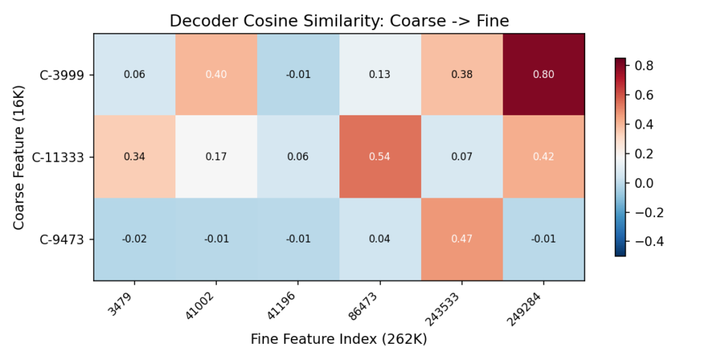
The Heatmap: Decoder Cosine Similarity
The heatmap shows the same data from a different angle. Each cell measures how much a coarse features and a fine features point in the same direction inside the model.
- High values mean they’re encoding the same thing at different zoom levels.
- Low values mean they’re unrelated.
| Coarse | Strongest Fine Match | Similarity | Reading |
|---|
| C-3999 | F-249284 | 0.80 | Near-identical direction. Almost certainly the same concept at different granularity |
| C-11333 | F-86473 | 0.54 | Strong overlap, plus two more matches at 0.42 and 0.34 |
| C-9473 | F-243533 | 0.47 | One clear sub-feature |
Values near zero mean unrelated. Above 0.3 is meaningful geometric correspondence.
The scatter plot
The scatter plot below shows every coarse-fine pair measured on both axes. X-axis is correlation, Y-axis is cosine similarity. Pairs in the upper-right quadrant (above 0.3 cosine, right of 0.5 correlation) are the real correspondences.
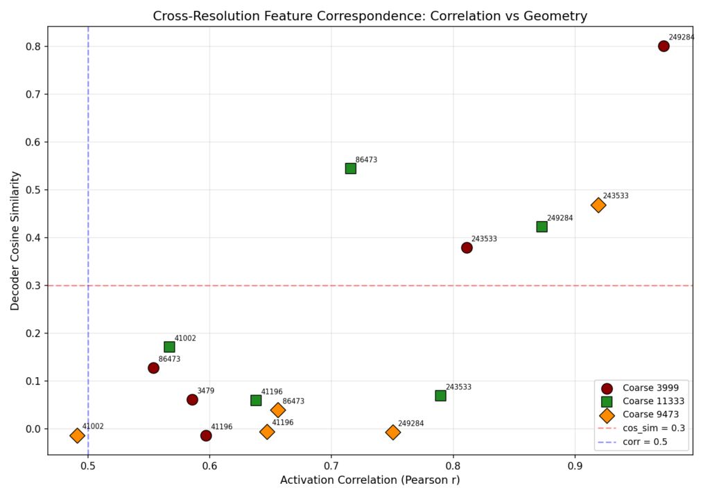
The strongest pair: C-3999 → F-249284, with correlation ~0.96 and cosine similarity 0.80. They fire on the same prompts AND point in the same direction. That’s as strong as cross-resolution correspondence gets.
Some pairs have high correlation but low cosine similarity (bottom-right area of the plot). Those feature
The Interpretation Gap
C-3999 gets labeled “France” because it reliably activates on France prompts and not on neutral ones. That’s standard practice in interpretability work. Label a feature by what activates it.
But the model doesn’t know the word “France.” It has a direction in 2304-dimensional space that, for whatever internal reason, turned out to be useful for predicting the next token when France-related patterns show up. We call it “France” because that’s the human category our test prompts were organized around. The model’s internal geometry might carve the world along boundaries that don’t align with our conceptual categories at all — we just can’t tell, because we only test with prompts organized around our categories.
| What we actually know | What we’re assuming |
|---|
| C-3999 fires on France prompts, not neutral | C-3999 “means” France |
| F-86473 fires on a subset of France prompts | F-86473 is a France sub-concept |
| C-3999 and F-249284 point in similar directions | They encode related meanings |
| Injecting C-3999’s direction changes output toward France-like text | The feature is causally involved in France generation |
The labels (“French cuisine,” “Paris landmarks”) are human interpretations based on which prompts activate a feature. The model doesn’t have those labels. It has frozen weights and an activation landscape that we’re projecting human categories onto.
Neural nets don’t memorize data. They find regularities and generalize those regularities to new data. A model will generate plausible text about unicorns even though it’s never seen one described as real, because it’s learned the relational structure of mythical creatures, horses, and horns. The internal representation that enables that generalization doesn’t need to map onto our concept of “unicorn.” It just needs to be useful for next-token prediction. When we label a feature “France,” we’re assuming the model’s useful regularity aligns with our semantic boundary. Sometimes it does. Sometimes we don’t know.
This is the wall that people like Neel Nanda keep writing about in mechanistic interpretability research. It was interesting to actually hit it myself. I can identify which features fire and when.
We can measure geometric relationships between them. But mapping that to human-readable meaning is always an inference, never ground truth.
When I started this project, I wanted/imagined i can build something like the Activation Space Navigator from the previous post using models real data.

Clean clusters with labeled regions you could point at and say “that’s France.”
The real data didn’t work that way. The 3D point cloud shows us directions in the model’s internal representation that reliably correlate with France-themed input.
Each feature in the SAE has a fixed direction inside the model, a “concept arrow” baked into the SAE’s weights. Feature C-3999’s arrow points in the direction the SAE learned to associate with France-related activation patterns.
When France text flows through Gemma, the residual stream at layer 12 aligns with that arrow. The SAE sees the alignment and says “this input has a big component along C-3999’s direction.” That’s the activation firing.
The arrows don’t move. The model’s state passes near them. Highway signs. Fixed in place, traffic passes by. France prompts pass close to certain signs. Neutral prompts don’t.
The 3D point cloud from the experiment projects these arrows into a space we can actually look at. Features that cluster together point in similar directions. Features that are far apart but still fire on the same prompts are the co-occurring concepts from the scatter plot’s bottom-right, related but geometrically distinct.
One thing worth naming: this is all an approximation. The SAE reconstructs the residual stream from its learned directions, and the reconstruction isn’t perfect. Some signal is always lost. We’re working with a useful approximation of the model’s internal state, not the thing itself.
So it’s not that “France activated these regions of the model’s weights.” The weights are frozen. The model has learned internal directions for France-related patterns, and when France text flows through, the residual stream aligns with those directions. That alignment is what we’re measuring.
Closing the loop
The previous post described system prompts as activation space manipulation.
This experiment confirmed it: the directions those prompts push activations toward are real, measurable, and decomposable into sub-features.
What’s Next for This Project
The activation mapping is done. I found real structure: coarse France features that decompose into fine sub-features, confirmed by both behavioral correlation and geometric similarity.
The GO/NO-GO question was whether the coarse-to-fine mapping would produce 3+ meaningful sub-features per coarse anchor. C-11333 has three above threshold. That’s a GO.
Phase 2 is the actual Steering Experiment.
Take those mapped features and test whether multi-resolution steering (coarse “France” + fine sub-features) produces better, more targeted output than single-resolution steering alone.
If it does, that’s evidence the cross-resolution structure isn’t just a statistical artifact. It’s a lever we can pull to tweak the behavior of a model
If it doesn’t, the structure is real but doesn’t actually control what the model generates. Correlation isn’t causation, even inside a neural network.
Either way, I’ll know more about what those frozen weights are actually doing when we hit enter.
References